Axel Paris

Adding Details to Implicit Surfaces

March 2, 2024 - Last updated: January 30, 2025

Adding details to implicit surfaces is challenging. As opposed to polygonal meshes, they do not provide an explicit parameterization of the surface which prevents the use of any texture mapping. The goal of this post is to investigate various techniques to workaround this issue and add details to implicit surfaces. Here We will focus on displacement mapping for implicit surfaces encoded as signed distance fields (SDF), whose field function `f \quad : \quad \mathbb R^3 \rightarrow \mathbb \R` returns an estimate of the distance to the surface of the object (see here for a more in-depth explanation). Everything written here can be tested in this shadertoy. These are mostly notes and code snippets for my future self which may be useful to other people.

The common approach for adding details is to combine the field function with procedural noise. This can be done in different ways, which we'll investigate here.

Noise-based details

The first, probably most straightforward technique (and most used!) to add details is to treat a 3D noise as a signed distance field itself, and combine it with the base SDF. You can see many examples of this in Shadertoy (here or here just to name a few). This is also referred to as hypertexturing in the research litterature. While such technique can theoretically add infinite details (to the extent of the number of octave you use), everything comes from the same noise function which suffers from a self-similar appearance. This may be partially solved by combining different functions depending in which region of space we evaluate it. Another downfall of this is that treating noise as a distance field everywhere will necessarily create floaters (detached surface parts floating in space), which is usually not desired.

Implicit sphere combined with 3D noise. As the amount of octaves increases, floaters appear (center and right images).
We can work around this issue if we refine the problem a little bit. Basic SDF primitives, such as spheres, capsules, and segments, are also often called skeletal primitives, and their signed distance function is made of a distance function to an infinitly-thin skeleton, and a substraction by a radius. Instead of adding noise to the global SDF as done before, we now add details to a given specific primitive by modifying its radius with noise. Let's study the case of a sphere, whose SDF is defined from a center `\mathbf{c}` and a radius `r` as:

`f(\mathbf{p}) = ||\mathbf{p} - \mathbf{c}|| - r`

Now let's make the radius also a function `r \quad : \quad\mathbb R^3 \rightarrow \mathbb \R` and define it using a noise `n \quad : \quad \mathbb R^3 \rightarrow \mathbb \R`:

`f(\mathbf{p}) = ||\mathbf{p} - \mathbf{c}|| - r(\mathbf{p})`

`r(\mathbf{p}) = r_b + a n({\pi(\mathbf{p})} / l)`

With `r_b` the base radius, `a` the noise amplitude, `l` the noise wavelength, and `\pi \quad : \quad \mathbb R^3 \rightarrow \mathbb \R^3` the projection function to the surface of the primitive (in this case a sphere). More precisely, the goal is to modify the radius of the primitive using a noise function - but this time, the evaluation is constrained to the surface of the primitive using the projection `\pi(\mathbf{p})`. This avoids the creation of floaters as the noise is not evaluated for every different point in 3D space but constrained to the sphere surface. This technique is also sometimes called star-shaped noise, and has been detailed in several papers (here, and more recently in one of my paper here).

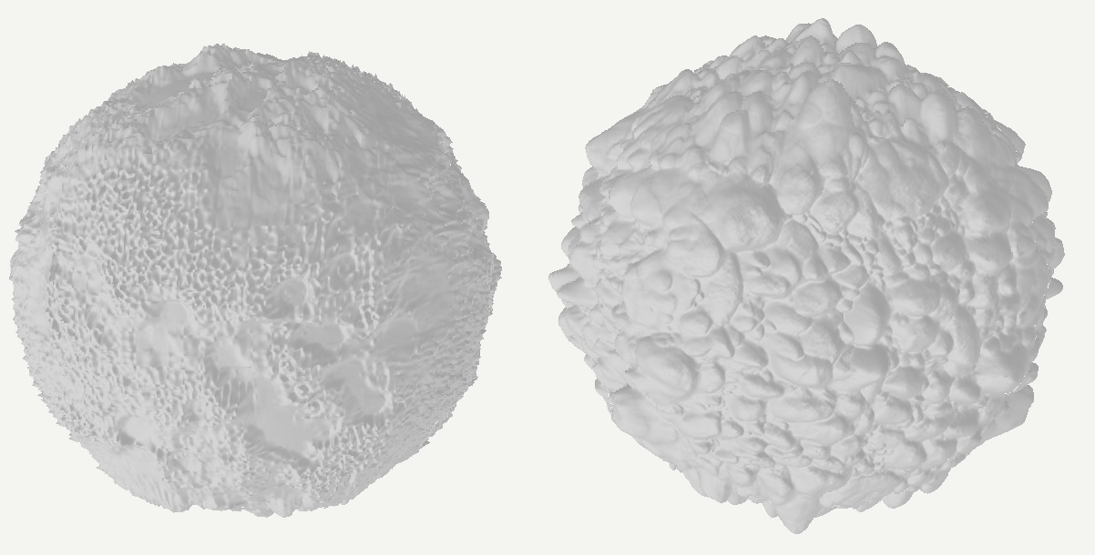
So-called star-shaped noise primitives ensure that there are no floaters in the scene. The noise evaluation is constrained to the surface of the underlying skeletal primitive.
This technique can be applied to any SDF that manipulate a radius. There are still some limitations. As opposed to hypertexturing presented above, star-shaped noise primitive cannot create overhangs on the shape, so the details appear a little more uniform. Details also come from the same noise function, which provides less expressivity and control than traditional texture mapping. Ideally we would want the same flexibility than meshes and displacement maps - which is not possible because of the lack of parameterization of implicit surfaces. Let's look into potential solutions.

Warping implicit surfaces

The closest equivalent of displacement for implicit surfaces is called warping. A warp is a domain deformation, and is widely used in computer graphics: for instance, image warping is commonly found in filters of messaging apps such as Snapchat to make your pictures look funny; in texture synthesis, warping is an essential tool to create procedural textures; and in implicit modeling, warping may be used to create more interesting shapes as it deforms space. In essence, a warp is a mapping `\mathbb R^3 \rightarrow \mathbb R^3` that is applied to the point before evaluating the SDF function. There are a lost of possible deformation, including affine transformation (translation, rotation, scale), bending, twisting (see here for more examples).

The problem is that we are still lacking a parameterization of our implicit surface (no UVs). So how can we parameterize our implicit primitives, and use it for warping? One classical UV-less pipeline used in the industry is triplanar mapping (also called box mapping), and it is possible to use this technique for warping implicit surfaces.

Triplanar warping

Triplanar mapping is a well-known technique for on-the-fly parameterization. A great reference from an article in GPU Gems 3 by Ryan Geiss is available online, and there are also detailed blog posts from Catlike Coding and Martin Palko, just to name a few. The idea is to use the world space position of a point `\mathbf{p}` and its normal `\mathbf{n}` to determine a parameterization. This has a big advantage: the surface you are trying to map to the texture does not need an explicit parameterization, which is perfect for implicit surfaces. The warping computed from the texture `T \quad : quad \mathbb R^3, \mathbb R^3 \rightarrow \mathbb \R^3` at a given point `\mathbf{p}` and normal `\mathbf{n}` (considering we sample a RGB texture) can be defined as:

`T(\mathbf{p}, \mathbf{n}) = \sum_{i=0}^{3} \alpha_i(\mathbf{n}) \cdot t \circ \gamma_i(\mathbf{p})`

The weighting function `\alpha_i` computes the contribution of each mapping of `\mathbf{p}` according to the dot product between the normal and the unit axis-aligned vectors: `\alpha_i(\mathbf{n}) = | \mathbf{n} \cdot u_i |`. The function `\gamma_i \quad : \quad \mathbb R^3 \rightarrow \mathbb R^2` computes the projection of `\mathbf{p}` on the i-th plane in world space and finally, the function `t \quad : quad \mathbb R^2 \rightarrow \mathbb \R` denotes the 2D function we want to map to our surface, and can be anything from a baked texture to a procedural noise.

If we interpret `t` as a function computing a color, then `T(mathbf{p}, \mathbf{n})` can be used to directly texture a implicit surfaces with albedo. Now what we can also do is deform the geometry of our implicit shape using triplanar warping. In this case, `t` is now a heightfield (or displacement map) and evaluting `T(mathbf{p}, \mathbf{n})` allows to compute the warping strength. As for the warping direction, we use the normal direction `\mathbf{n}` from which we computed our weighting coefficients. The final warping function `w` is then defined as:

`w(\mathbf{p}) = \mathbf{p} - \mathbf{n} \cdot T(\mathbf{p}, \mathbf{n}) `

Then, the new implicit function `\tilde{f}` is defined as the composition of the base shape function `f` and the warping operator:

`\tilde{f}(p) = f \circ w(p)`

As with star-shaped noise, triplanar warping is applied to a specific primitive or subset of primitives - a sphere in the following figure.

Implicit spheres warped with different textures.

While this technique is powerful, it also has several limitations. First, a requirement is that the normal should be continuous. Discontinuities in normals will lead to discontinuities in the warping, which in turn will create holes in the object itself. A typical failure case is a sharp box primitive - we would need a rounded box for the operator to work without visual artifacts, as it provides smooth normals over the entire primitive. Another thing worth mentioning is that it is computationally expensive: triplanar mapping in general is not free, and warping is also known to be expensive in implicit modeling. One could investigate the use of biplanar mapping to save some computations.

Using this technique also not only break the Euclidean distance property of the SDF (as it is the case for most operations), but is also far from being gentle on the Lipschitz constant of the function (the upper bound of the norm of the gradient, which is 1 for SDF, and is less than 1 known for conservative SDFs). The actual Lipschitz constant remains to be computed in this case, but you'll need to divide your sphere tracing steps for the final rendering to be artifacts free. This is also the case for the other two methods presented in this post, but to a lesser extent.

All results presented in this post can be explored in this shadertoy.

Implicit spheres amplified with details from the three different techniques presented in this post, namely hypertexturing (left), star-shaped noise (center) and triplanar warping (right).

References

Wyvill - The Blob Tree - Warping, Blending and Boolean Operations

Implicit Sweep Objects

ScratchAPixel - Rendering Distance Fields

Ryan Geiss - Generating Complex Procedural Terrains Using the GPU

Inigo Quilez - 3D Distance functions